TOC is about maximizing flow through a system.

The analogy that Dr. Goldratt used was a chain:  A chain resists as much as its weakest link.

The weakest link determines the MAXIMUM flow a system can produce (however the flow is produced by the interaction of all the parts of the system, so all of them are important - this clarifying note is to erradicate the false notion that TOC would say "only the constraint is important").

The weakest link is what we call the constraint. Formally, a constraint is an element of the system that limits throughput generation.

Definition of SYSTEM: A set of interdependent elements with a purpose (or goal).

Definition of three terms to describe what happens in a system:

THROUGHPUT: units of the goal produced per unit of time through the operation of the system.

INVENTORY: amount of money captured in the system to produce throughput (usually raw materials and equipment).

OPERATING EXPENSE: amount of money to operate the system per unit of time.

Understanding the system with these three terms changes profoundly the base on what decisions are made today in the majority of companies. There are two wide spread notions that block managers from making better operational decisions:

1) Cost accounting: it is intended to measure the cost and make better decisions, but actually cost accounting is enemy n°1 of productivity for all the distorsions it introduces in decision making. Contact us asking for more details if you want to know more about our views on this subject.

2) Waste elimination: it sounds reasonable that eliminating waste we can improve productivity. However, when we understand that we need to maximize throughput of the system as a whole, and due to uncertainty and natural variation we need buffers to protect flow, we understand that many of the so called wastes are buffers. Therefore, reducing waste as an objective will reduce necessary buffers most of the time (it is our experience). All the improvement programs aimed to reduce waste are enemy n°2 of productivity.

You will find reasonable amount of logic and science to substantiate these two (strong and bold) statements in the next sections of this page.

OTIF100 is disruptive because will suggest decisions that contradict common knowledge or "best practices".

If we want to balance our flow, we need to unbalance our line. In other words, once we have decided (or found) our constraint, the rest of the resources MUST have more capacity.

Please, go and learn with the dice game what happens when we balance the capacity throughout a production line. And please, don't balance your line. The dice game is described in The Goal, chapter 14.

The Dice Game 

OTIF100 is a system to help MTO - Make To Order companies achieve the best due date Performance ~ 100%. As a necessary condition, we will make a decision to achieve the maximum throughput possible through the system.

Let us define a term. WIP: work in progress, is the amount of orders that are currently being processed by the line.

A work order that is accepted and ready to be processed but we haven't allowed to enter the line yet is not WIP.

The main concept is that WIP is a major factor in the actual capacity of our line. The two extremes are harmful:

The first case is if we have very little WIP, then we will produce very little. This is obvious... (and yet, OPF - One Piece Flow pushes the system to this extreme, but OPF is regarded as an objective by some methodologies... yes, we are disruptive).

The second case is if we allow too much WIP, then flow goes slower, producing less than if the WIP was less.

An analogy will help understand better: a highway is a production system. If we place a flag at a certain point and we count vehicles per minute passing by the flag, we will have a good measurement of the capacity of the highway. If we allow only one car per hour, no matter the speed, the highway will produce only one car per hour. Now, if we allow a great amount of cars -remember those days starting a holiday- and we measure again, due to the slow speed, the capacity will be low. If we could tell the drivers to park for half an hour if, for example, their plates end in an odd number, half of the cars would flow much faster, hence producing more vehicles per hour. Note that the parked vehicles will move much faster half an hour later, so they also will arrive earlier to destination.

The analogy of the highway shows how WIP determines the actual capacity of the system. Furthermore, as most companies don't control WIP, the fluctuations will result in daily throughput so variable that we cannot predict anymore when an order will be finished, therefore it is very unlikely that we can meet our promises of delivery time with high certainty. And worse, in the attempt of improving service, we continuously go changing priorities in production, reducing even more both capacity and quality.

 Let us use the promised due dates to decide how much WIP to allow in our line. As we don't know your operation, the only thing we can suggest here is a generic rule of thumb that has worked every single time that we applied it.

Surely you have a standard lead time to promise each order. This is a lead time that is accepted by the market because your competitors are not far from offering the same delivery times. We will use this time as our first input and we will call it SDT - Standard Delivery Time, and it will be a number of days.

It is safe to assume that you promised that time based on your experience of how many days it took you to produce similar products. Recalling the highway analogy, we will introduce here the concept of PBT - PRODUCTION BUFFER TIME to be half of SDT.

You may have noticed that there are groups of products in your portfolio that take more or less the same time to finish, so we can group the products in Production Families. The rule of thumb here is that a family is diferent from another when the buffer is different in 25% or more. For example, it doesn't make sense to have two families with 9 days and 11 days. It starts to make sense if they were 9 and 12.

The main criterion to separate products into more than one family is the routing and complexity of the product. It is not the speed of processing, even at the constraint. This will give us another measurement to make commercial decisions (ask us if you are interested), but not operational ones.

Typically we can end up with two or three production buffer times, and you may decide to have more families even if they share the same PBT. All our products (SKU - stock keeping units) must belong to a production family, to assign the PBT to the order.

Finally, we introduce here another concept: SRD - SCHEDULED RELEASE DATE. We say an order is released when it is allowed to be processed. SRD is computed based on the PDD - Promised Due Date and PBT:

        SRD = PDD - PBT

We call it Scheduled to distinguish it from ARD - Actual Release Date, which is the date where the order was actually released. When ARD is earlier than SRD, we are allowing more WIP than recommended by these rules and most likely clogging our line (except if released using Load Control). When ARD is later than SRD, we are reducing the probability of delivering on time. In the latter case we say that we are eating on the buffer without producing.

WIP CONTROL is simply releasing WIP on the SRD. (See Load Control for releasing before SRD).

THE LIST OF SCHEDULED RELEASE DATES IS OUR PLAN.

NOTE 1: All the calculations are considering working days. In OTIF100 there is a calendar of NWD - Non Working Days so all the calculations will consider only working days.

NOTE 2: As delivery times are often given in calendar days, the PBT should consider this. For example, if you usually promise 30 calendar days and you work from Monday to Friday, the PBT should be something between 10 and 12 days, because these will be working days, equivalent to ~15 calendar days.

NOTE 3: In the tutorials we mention the concept of FULL KIT. It is very likely that an order must be interrupted because we lack some tool or material in the middle of the process. This is a disruption that we want to avoid. FULL KIT is the set of preparations to complete an order. The best practice is to ensure FULL KIT before releasing any order. The time between the sale and the SRD is a perfect time to ensure FULL KIT without any urgency.

NOTE 4: The rule of thumb given to calculate PBT is half of regular delivery time promised. If your business is to promise several weeks or months in advance, in this case consider the production lead time at full capacity that you had in the past and divide this by half.

 Once we have our Production Families with their respective PBT, we can design a robust yet simple priority system.

First, we need a priority system so the workers can decide what order to process next. If this decision depends on a supervisor or a manager, it takes too much time and occasionally is wrong (otherwise there would be no changes, right?). So we better design a good system that never changes and let the workers work well in the right sequence.

Let us remember that we want to achieve 100% Due Date Performance, to have a perfect OTIF - On Time In Full. So the first idea would be to use due dates as our criterion to set priorities. See the example in the table:

Work Order	Product SKU	Promised Due Date
WO-01	P1	MAY, 5
WO-02	P3	MAY, 6
WO-03	P2	MAY, 7
WO-04	P1	MAY, 8
WO-05	P3	MAY, 9
WO-06	P2	MAY, 10
WO-07	P2	MAY, 11
WO-08	P1	MAY, 12

If we decide to use PDD as the only criterion and we have all these orders in front of our work center, we should process P1, make a setup, then P3, make a setup, then P2, make a setup, again P1, and so on.

We all know how setups can eat up on the available time to produce. It is a real waste to spend more time in setups than necessary.

On the other hand, if our delivery time is, say 30 days, processing WO-02 before WO-01 will not do a difference. So now we are forced to violate our priority system for good reasons, ending in the same unpleasant place where we started: with no clear priority system.

The way out is to use the PBT as our best indicator to decide on the priority of a certain order: the closer the due date, the higher the prority, but similar priorities should be equal in value, so the worker can decide on a simple rule what to do next.

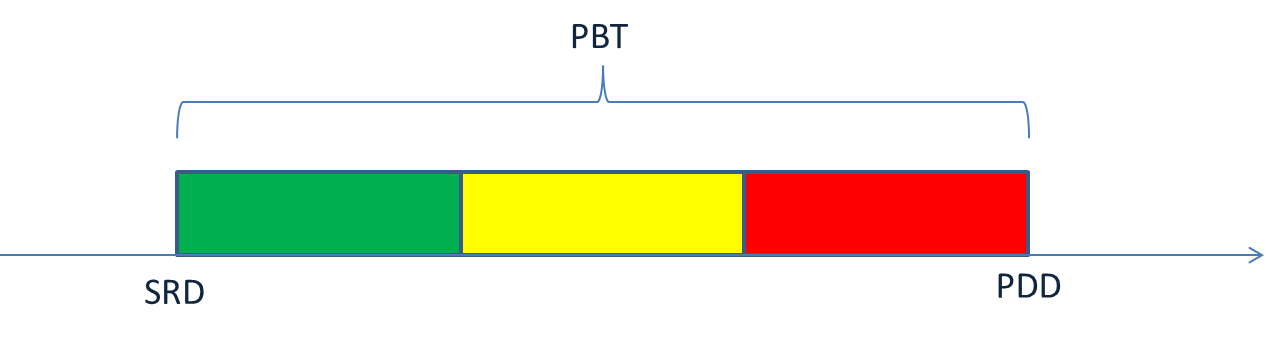
Production Buffer Time - PBT is the time between PDD and SRD. We can divide it in three equal zones, each of them grouping similar priorities. If we paint with a color each zone, we can have a simple priority system based on colors. These are four colors (later than PDD is late and we need a color for those):

PRIORITY	COLOR
Urgent - Late	0. black
Highest	1. red
Medium	2. yellow
Lowest	3. green

In OTIF100 you will see the colors in the list of orders and each work order will show the words as in this table.

Applying this to the orders of our example, let's imagine we are looking at our orders on May 2:

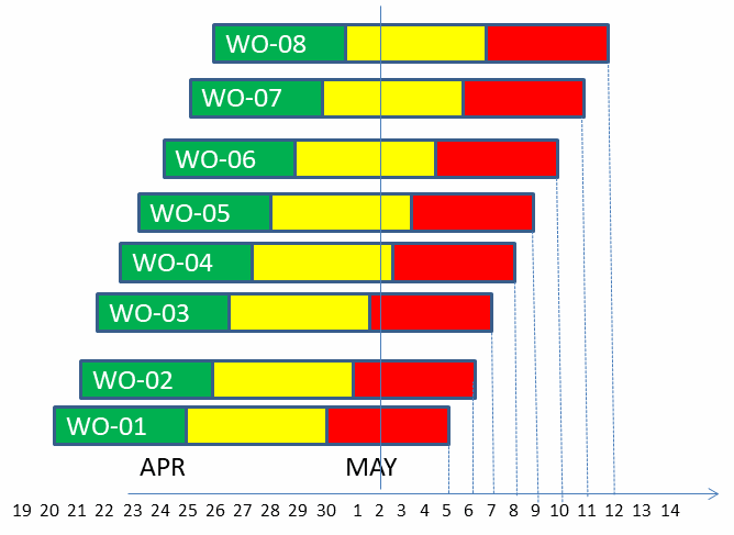Now we know orders WO-01, WO-02 and WO-03 have the highest priority but we can choose either one without causing any problem to DDP. So the decision, based on colors and setups, could be:

WO-01, setup, WO-02, setup, WO-03, WO-06, WO-07, setup, WO-04, WO-08, setup, WO-05

Maybe, you could figure out a better sequence. The one who probably will have better information, intuition and experience to decide the best sequence is the worker, so we give them a simple rule: follow the colors, within the same color, do as you think best. And we let them work.

THE COLOR SYSTEM IS OUR EXECUTION CONTROL SYSTEM.

NOTE: In OTIF100 you will see orders with color 4. cyan which is the color for orders that shouldn't be released. As managers could decide to release an order anyway, the orders released earlier than SRD are painted green because you may have released earlier with Load Control signals. If you don't have Load Control yet, it is better to release on SRD.

When sales grow, demand over your capacity may consume even the revealed capacity with the initial method. It is time to implement the Load Control mechanism of OTIF100.

Load Control will allow you to make two decisions that will enhance your ability of meeting promised due dates:
1. Estimation of due dates based on actual load. This estimation is more accurate and increase probability of delivering on the promise to the customers. It assumes that actual capacity will not vary out of range, which what happens when WIP is out of control.
2. Decide when to release earlier, improving utilization of your capacity. Sales follow an irregular pattern, it is very likely that orders will be scheduled to release more some days than others. When this concentration is too much for some days and too little for others, we have a negative fluctuation of WIP. Production line status shows load and advice on releasing some orders earlier or not.

Configuration takes significantly more time and it may require some time with our experts over an online meeting. The difficulty is to estimate parts per hour in the decided resources, which may take some days in front of the chosen CCRs.

The main concept of Theory Of Constraints is that a chain of processes cannot move faster than the slowest element (a chain can resist only up to the resistance of the weakest link).

We will call CCR any resource that is close to the minimum capacity or slowest pace of production. When WIP is controlled, accumulation of WIP occurs in front of CCRs. See Balanced flow paragraph to learn why it is better to have "protective capacity" in most resources. These are not CCRs. In fact, the ideal is to have only one CCR.

The CCR that is the constraint of a production line in a given period is what we call Flow Dictator, and it is the resource that governs the flow.

Sometimes, there are SKUs that go faster through one CCR than through another. So depending on the mix of SKUs and quantities, one CCR can be flow dictator during a period and may shift to the other in the next period.

Our advice is to add capacity to one of those and keep flow dictator in the same place (remember you can add capacity extending working hours). However, when differences with different mixes are significant, OTIF100 allows three CCRs to be included in calculations, so flow dictator will be identified automatically to give the right signals to production.

The best way to measure capacity in a certain resource is measuring utilized time for a batch, and then divide parts produced in that measured period. For example: a batch of three parts took four hour and twenty minutes. Parts per hour PPH = 3 / 4.33 = 0.6928. Once we have a good enough sample of measures with all different SKUs, we can make a table with rounded PPH values. For example, 0.69 can be close to 0.60 or 0.80. And all similar SKUs will have same value to PPH. This is a good practice to include very quickly a new product in our list.

Note: there is no need to calculate anything accurately. Remember that we have buffers to absorb small variations, than average out, so we cannot have an accurate measure anyway. Disregard setup times as well: DDP is the primary objective, thus setup must be subordinated to it. See Color Priority System for more details.

Available capacity is then expressed in working days, and we can measure how this capacity is filled using the quantities and PPH, along with the hours per day assigned to that resource.

If we knew when we are going to deliver an order, promising that date would ensure a high Due Date Performance or ~ 100% OTIF (On Time In Full).

Why most companies have DDP below 85% - 90%? Wait... an 85% DDP is considered very high in some companies (no names here, but it is a fact). Even they considered 85% as a theoretical limit that cannot be surpassed without a high cost.

And let us understand something about DDP. For the customer, 85% is poor: it is the same probability of surviving Russian roulette. Not even 90% is a good performance. A customer waiting for a delivery of a material for his own production, the cost of delay is much higher than the cost of the goods. So guaranteeing 100% DDP creates a highly valuable proposition to the market.

We believe that all manufacturers know this. Why can't they achieve such performance? We discard that they don't want to improve their service. The answer must be that they are not sure of the date the order can be finished. They have an estimate, but they also know about Murphy's law and unexpected circumstances that delay some orders... it's life! Our hypothesis is that WIP fluctuation produces actual capacity fluctuation, so all the delivery times move accordingly, many times beyond the boundaries of estimations (as good intended as they were).

The solution in OTIF100 is to first take control of WIP. Once the production line is stable, we can measure approximately how many parts per hour the flow dictator will produce of each SKU. Having this number, we can estimate how many hours will all the accepted orders take to be produced, and we translate this to working days. Now we can assess when it is more likely that the next order can be delivered. And we add half of PBT (production buffer time) to that date and we have produced a high probability or safe delivery date, being this date within the acceptable lead times by the market.

As flow dictator can move from one CCR to another depending on the mix, OTIF100 makes the estimation for a certain mix of production dinamically.

Good service is fulfilling the promise given to the market.

The promise with MTO is to deliver on the promised date.

The promise with MTA is to have availability for immediate delivery.

MTA keeps a buffer of inventory for each SKU where the objective is to never run out while keeping the least possible inventory. For each SKU, we establish a stock buffer and we only trigger a production order when there is a consumption of that buffer. (See more details in www.fillrate100.com).

This means that orders for MTO can be accepted or rejected for some date, whereas MTA orders are triggered, accepted and released upon consumption.

When the company has a business with a mixture of MTO and MTA, the dilemmas are: how to promise a date when we don't know if we will have the capacity to fullfill it (MTA orders may use the needed capacity for MTO), and also how to decide on the priorities when MTO and MTA orders compete for the same resource.

The solution for these two dilemmas is to separate capacity for MTO and MTA in the planning phase, so when we launch orders, they will have enough capacity in all cases.

We can estimate how much capacity of the CCR will be used on average for MTA orders (use historical data or just an estimation). Then add a capacity buffer to this estimation. The remainder can be used in the load control mechanism to promise dates for MTO orders.

Example:

Suppose we manufacture towels. We can make different SKUs to sell in stores, so this is MTA. But we can also take orders from hotels, with special designs, and these are MTO.

We can estimate how many hours per month it is used to replenish MTA buffers and calculate what percentage of the total hours in the month is that. Let us say it is 30%. As MTO orders are not flexible, we better allow for a cushion between the two capacities, so we assign an additional 20% to MTA, so we reserve 36% to MTA. In OTIF100 this means assigning 64% to MTO in load control.

To load MTA orders to OTIF100 we must include stock buffer and on hand, so the MTA order will show the corresponding color, solving the second dilemma. Both MTO and MTA orders now have colors, so the priority system doesn't change.

The expected behaviour is that both MTO and MTA orders will flow in the right sequence without clashing.

In load control we have the target WIP horizon.

We already know that looking at the load within this horizon, we can decide to release more MTO orders.

Now that we have a reserved capacity, OTIF100 will show the load as usage of the reserved capacity within the target horizon.

Beneath that, OTIF100 shows the usage of the reserved capacity for MTA because of the load of MTA orders. When this number is over 100%, it is red as an alert. 

If you have red loads in MTA for a long time, it is unavoidable that either some MTO orders will be late or some SKUs will run out of stock. A healthy system keeps this load between 80% and 100%.